Spline Interpolant PtByPt VI

Owning Palette: Interpolation PtByPt VIs

Requires: Full Development System

Returns an array, Interpolant, of length n.

The array contains the second derivatives of the spline interpolating function g(x) at the tabulated points , where i = 0, 1, …, n – 1.

Note  By default, reentrant execution is enabled in all Point By Point VIs.

This VI is similar to the Spline Interpolant VI.

Details  Example

Add to the block diagram

Find on the palette

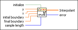
	initialize, when TRUE, initializes the internal state of the VI.
	y is an input data point.
	x is an input data point.
	initial boundary is the first derivative of interpolating function g(x) at x[0], g'(x[0]). The default is 1.0E+30, which causes this VI to set the initial boundary condition for a natural spline.
	final boundary is the first derivative of interpolating function g(x) at x[n – 1], g'(x[n – 1]). The default is 1.0E+30, which causes this VI to set the final boundary condition for a natural spline.
	sample length is the length of each set of incoming data. The VI performs computation for each set of data. The default is 100. sample length must be greater than zero.
	Interpolant is the second derivative of interpolating function g(x) at points x[i], i = 0, 1, …, n – 1.
	error returns any error or warning from the VI. You can wire error to the Error Cluster From Error Code VI to convert the error code or warning into an error cluster.

Spline Interpolant PtByPt Details

The sets of input data x and y have length n and contain a tabulated function, f(x_i) = y_i, with x₀ < x₁ <…x_{n – 1}. initial boundary and final boundary are the first derivatives of the interpolating function g(x) at points 0 and n – 1, respectively.

Example

Refer to the Spline Interpolation PtbyPt VI in the labview\examples\Signal Processing\Point by Point directory for an example of using the Spline Interpolant PtByPt VI.

 Open example  Find related examples