|
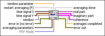
window parameter specifies the beta parameter for a Kaiser window, the standard deviation for a Gaussian window, and the ratio, s, of the main lobe to the side lobe for a Dolph-Chebyshev window. If window is any other window, this VI ignores this input.
The default value of window parameter is NaN, which sets beta to 0 for a Kaiser window, the standard deviation to 0.2 for a Gaussian window, and s to 60 for a Dolph-Chebyshev window.
|
 |
restart averaging specifies whether the VI restarts the selected averaging process. If restart averaging is TRUE, the VI restarts the selected averaging process. If restart averaging is FALSE, the VI does not restart the selected averaging process. The default is FALSE. When you call this VI for the first time, the averaging process restarts automatically. A typical case when you should restart averaging is when a major input change occurs in the middle of the averaging process.
|
 |
time signal X is the time waveform X.
|
|
time signal Y is the time waveform Y.
|
 |
window (Hanning) is the time-domain window to apply to the time signal. The default window is Hanning.
| 0 | Rectangle | | 1 | Hanning (default) | | 2 | Hamming | | 3 | Blackman-Harris | | 4 | Exact Blackman | | 5 | Blackman | | 6 | Flat Top | | 7 | 4 Term B-Harris | | 8 | 7 Term B-Harris | | 9 | Low Sidelobe | | 11 | Blackman Nutall | | 30 | Triangle | | 31 | Bartlett-Hanning | | 32 | Bohman | | 33 | Parzen | | 34 | Welch | | 60 | Kaiser | | 61 | Dolph-Chebyshev | | 62 | Gaussian |
|
 |
error in describes error conditions that occur before this node runs. This input provides standard error in functionality.
|
 |
averaging parameters is a cluster that defines how the averaging is computed. The specifications of the parameters include the type of averaging, the type of weighting, and the number of averages.
 |
averaging mode specifies the averaging mode.
| 0 | No averaging (default) | | 1 | Vector averaging | | 2 | RMS averaging | | 3 | Peak hold |
|
|
weighting mode specifies the weighting mode for RMS and vector averaging.
| 0 | Linear | | 1 | Exponential (default) |
|
|
number of averages specifies the number of averages used for RMS and vector averaging. If weighting mode is exponential, the averaging process is continuous. If weighting mode is linear, the averaging process stops after this VI computes the selected number of averages.
|
|
|
FRF mode specifies how to compute the frequency response function (FRF). If you know that noise, which does not propagate through the system under test, infiltrates the input or output signals, you can select the method used for computing the frequency response function (H1, H2, H3) to minimize the measurement error.
| 0 | H1 (default)—Select H1 to minimize errors in the result when extraneous noise contaminates the output signal. | | 1 | H2—Select H2 to minimize errors in the result when extraneous noise contaminates the input signal. | | 2 | H3—When noise contaminates both the input and output signals, H1 and H2 provide the lower and upper bounds of the true frequency response of the system. In this case, select H3, the average of H1 and H2. |
|
 |
averaging done returns TRUE when averages completed is greater than or equal to the number of averages specified in averaging parameters. Otherwise, averaging done returns FALSE. averaging done is always TRUE if the selected averaging mode is No averaging.
|
 |
real part returns the real part of the averaged frequency response and the frequency scale.
 |
f0 returns the start frequency, in hertz, of the spectrum.
|
|
df returns the frequency resolution, in hertz, of the spectrum.
|
 |
real part is the real part of the averaged frequency response.
|
|
|
imaginary part returns the imaginary part of the averaged frequency response and the frequency scale.
|
f0 returns the start frequency, in hertz, of the spectrum.
|
|
df returns the frequency resolution, in hertz, of the spectrum.
|
|
imaginary part is the imaginary part of the averaged frequency response.
|
|
|
coherence returns the coherence and the frequency scale.
|
f0 returns the start frequency, in hertz, of the spectrum.
|
|
df returns the frequency resolution, in hertz, of the spectrum.
|
|
coherence returns the coherence.
|
|
|
averages completed returns the number of averages completed by the VI at that time.
|
 |
error out contains error information. This output provides standard error out functionality.
|
|
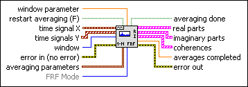
window parameter specifies the beta parameter for a Kaiser window, the standard deviation for a Gaussian window, and the ratio, s, of the main lobe to the side lobe for a Dolph-Chebyshev window. If window is any other window, this VI ignores this input.
The default value of window parameter is NaN, which sets beta to 0 for a Kaiser window, the standard deviation to 0.2 for a Gaussian window, and s to 60 for a Dolph-Chebyshev window.
|
|
restart averaging specifies whether the VI restarts the selected averaging process. If restart averaging is TRUE, the VI restarts the selected averaging process. If restart averaging is FALSE, the VI does not restart the selected averaging process. The default is FALSE. When you call this VI for the first time, the averaging process restarts automatically. A typical case when you should restart averaging is when a major input change occurs in the middle of the averaging process.
|
|
time signal X is the time waveform X.
|
 |
time signals Y is the array of time waveforms Y.
|
|
window (Hanning) is the time-domain window to apply to the time signal. The default window is Hanning.
| 0 | Rectangle | | 1 | Hanning (default) | | 2 | Hamming | | 3 | Blackman-Harris | | 4 | Exact Blackman | | 5 | Blackman | | 6 | Flat Top | | 7 | 4 Term B-Harris | | 8 | 7 Term B-Harris | | 9 | Low Sidelobe | | 11 | Blackman Nutall | | 30 | Triangle | | 31 | Bartlett-Hanning | | 32 | Bohman | | 33 | Parzen | | 34 | Welch | | 60 | Kaiser | | 61 | Dolph-Chebyshev | | 62 | Gaussian |
|
|
error in describes error conditions that occur before this node runs. This input provides standard error in functionality.
|
|
averaging parameters is a cluster that defines how the averaging is computed. The specifications of the parameters include the type of averaging, the type of weighting, and the number of averages.
|
averaging mode specifies the averaging mode.
| 0 | No averaging (default) | | 1 | Vector averaging | | 2 | RMS averaging | | 3 | Peak hold |
|
|
weighting mode specifies the weighting mode for RMS and vector averaging.
| 0 | Linear | | 1 | Exponential (default) |
|
|
number of averages specifies the number of averages used for RMS and vector averaging. If weighting mode is exponential, the averaging process is continuous. If weighting mode is linear, the averaging process stops after this VI computes the selected number of averages.
|
|
|
FRF mode specifies how to compute the frequency response function (FRF). If you know that noise, which does not propagate through the system under test, infiltrates the input or output signals, you can select the method used for computing the frequency response function (H1, H2, H3) to minimize the measurement error.
| 0 | H1 (default)—Select H1 to minimize errors in the result when extraneous noise contaminates the output signal. | | 1 | H2—Select H2 to minimize errors in the result when extraneous noise contaminates the input signal. | | 2 | H3—When noise contaminates both the input and output signals, H1 and H2 provide the lower and upper bounds of the true frequency response of the system. In this case, select H3, the average of H1 and H2. |
|
|
averaging done returns TRUE when averages completed is greater than or equal to the number of averages specified in averaging parameters. Otherwise, averaging done returns FALSE. averaging done is always TRUE if the selected averaging mode is No averaging.
|
 |
real parts returns an array of the real parts of the averaged frequency responses and the frequency scales.
|
f0 returns the start frequency, in hertz, of the spectrum.
|
|
df returns the frequency resolution, in hertz, of the spectrum.
|
|
real part is the real part of the averaged frequency response.
|
|
|
imaginary parts returns an array of the imaginary parts of the averaged frequency responses and the frequency scales.
|
f0 returns the start frequency, in hertz, of the spectrum.
|
|
df returns the frequency resolution, in hertz, of the spectrum.
|
|
imaginary part is the imaginary part of the averaged frequency response.
|
|
|
coherences returns an array of the coherence functions of the averaged frequency responses and the frequency scales.
|
f0 returns the start frequency, in hertz, of the spectrum.
|
|
df returns the frequency resolution, in hertz, of the spectrum.
|
|
coherence returns the coherence.
|
|
|
averages completed returns the number of averages completed by the VI at that time.
|
|
error out contains error information. This output provides standard error out functionality.
|
|
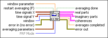
window parameter specifies the beta parameter for a Kaiser window, the standard deviation for a Gaussian window, and the ratio, s, of the main lobe to the side lobe for a Dolph-Chebyshev window. If window is any other window, this VI ignores this input.
The default value of window parameter is NaN, which sets beta to 0 for a Kaiser window, the standard deviation to 0.2 for a Gaussian window, and s to 60 for a Dolph-Chebyshev window.
|
|
restart averaging specifies whether the VI restarts the selected averaging process. If restart averaging is TRUE, the VI restarts the selected averaging process. If restart averaging is FALSE, the VI does not restart the selected averaging process. The default is FALSE. When you call this VI for the first time, the averaging process restarts automatically. A typical case when you should restart averaging is when a major input change occurs in the middle of the averaging process.
|
|
time signals X is the array of time waveforms X.
|
|
time signal Y is the time waveform Y.
|
|
window (Hanning) is the time-domain window to apply to the time signal. The default window is Hanning.
| 0 | Rectangle | | 1 | Hanning (default) | | 2 | Hamming | | 3 | Blackman-Harris | | 4 | Exact Blackman | | 5 | Blackman | | 6 | Flat Top | | 7 | 4 Term B-Harris | | 8 | 7 Term B-Harris | | 9 | Low Sidelobe | | 11 | Blackman Nutall | | 30 | Triangle | | 31 | Bartlett-Hanning | | 32 | Bohman | | 33 | Parzen | | 34 | Welch | | 60 | Kaiser | | 61 | Dolph-Chebyshev | | 62 | Gaussian |
|
|
error in describes error conditions that occur before this node runs. This input provides standard error in functionality.
|
|
averaging parameters is a cluster that defines how the averaging is computed. The specifications of the parameters include the type of averaging, the type of weighting, and the number of averages.
|
averaging mode specifies the averaging mode.
| 0 | No averaging (default) | | 1 | Vector averaging | | 2 | RMS averaging | | 3 | Peak hold |
|
|
weighting mode specifies the weighting mode for RMS and vector averaging.
| 0 | Linear | | 1 | Exponential (default) |
|
|
number of averages specifies the number of averages used for RMS and vector averaging. If weighting mode is exponential, the averaging process is continuous. If weighting mode is linear, the averaging process stops after this VI computes the selected number of averages.
|
|
|
FRF mode specifies how to compute the frequency response function (FRF). If you know that noise, which does not propagate through the system under test, infiltrates the input or output signals, you can select the method used for computing the frequency response function (H1, H2, H3) to minimize the measurement error.
| 0 | H1 (default)—Select H1 to minimize errors in the result when extraneous noise contaminates the output signal. | | 1 | H2—Select H2 to minimize errors in the result when extraneous noise contaminates the input signal. | | 2 | H3—When noise contaminates both the input and output signals, H1 and H2 provide the lower and upper bounds of the true frequency response of the system. In this case, select H3, the average of H1 and H2. |
|
|
averaging done returns TRUE when averages completed is greater than or equal to the number of averages specified in averaging parameters. Otherwise, averaging done returns FALSE. averaging done is always TRUE if the selected averaging mode is No averaging.
|
|
real parts returns an array of the real parts of the averaged frequency responses and the frequency scales.
|
f0 returns the start frequency, in hertz, of the spectrum.
|
|
df returns the frequency resolution, in hertz, of the spectrum.
|
|
real part is the real part of the averaged frequency response.
|
|
|
imaginary parts returns an array of the imaginary parts of the averaged frequency responses and the frequency scales.
|
f0 returns the start frequency, in hertz, of the spectrum.
|
|
df returns the frequency resolution, in hertz, of the spectrum.
|
|
imaginary part is the imaginary part of the averaged frequency response.
|
|
|
coherences returns an array of the coherence functions of the averaged frequency responses and the frequency scales.
|
f0 returns the start frequency, in hertz, of the spectrum.
|
|
df returns the frequency resolution, in hertz, of the spectrum.
|
|
coherence returns the coherence.
|
|
|
averages completed returns the number of averages completed by the VI at that time.
|
|
error out contains error information. This output provides standard error out functionality.
|
|
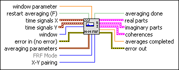
window parameter specifies the beta parameter for a Kaiser window, the standard deviation for a Gaussian window, and the ratio, s, of the main lobe to the side lobe for a Dolph-Chebyshev window. If window is any other window, this VI ignores this input.
The default value of window parameter is NaN, which sets beta to 0 for a Kaiser window, the standard deviation to 0.2 for a Gaussian window, and s to 60 for a Dolph-Chebyshev window.
|
|
restart averaging specifies whether the VI restarts the selected averaging process. If restart averaging is TRUE, the VI restarts the selected averaging process. If restart averaging is FALSE, the VI does not restart the selected averaging process. The default is FALSE. When you call this VI for the first time, the averaging process restarts automatically. A typical case when you should restart averaging is when a major input change occurs in the middle of the averaging process.
|
|
time signals X is the array of time waveforms X.
|
|
time signals Y is the array of time waveforms Y.
|
|
window (Hanning) is the time-domain window to apply to the time signal. The default window is Hanning.
| 0 | Rectangle | | 1 | Hanning (default) | | 2 | Hamming | | 3 | Blackman-Harris | | 4 | Exact Blackman | | 5 | Blackman | | 6 | Flat Top | | 7 | 4 Term B-Harris | | 8 | 7 Term B-Harris | | 9 | Low Sidelobe | | 11 | Blackman Nutall | | 30 | Triangle | | 31 | Bartlett-Hanning | | 32 | Bohman | | 33 | Parzen | | 34 | Welch | | 60 | Kaiser | | 61 | Dolph-Chebyshev | | 62 | Gaussian |
|
|
error in describes error conditions that occur before this node runs. This input provides standard error in functionality.
|
|
averaging parameters is a cluster that defines how the averaging is computed. The specifications of the parameters include the type of averaging, the type of weighting, and the number of averages.
|
averaging mode specifies the averaging mode.
| 0 | No averaging (default) | | 1 | Vector averaging | | 2 | RMS averaging | | 3 | Peak hold |
|
|
weighting mode specifies the weighting mode for RMS and vector averaging.
| 0 | Linear | | 1 | Exponential (default) |
|
|
number of averages specifies the number of averages used for RMS and vector averaging. If weighting mode is exponential, the averaging process is continuous. If weighting mode is linear, the averaging process stops after this VI computes the selected number of averages.
|
|
|
FRF mode specifies how to compute the frequency response function (FRF). If you know that noise, which does not propagate through the system under test, infiltrates the input or output signals, you can select the method used for computing the frequency response function (H1, H2, H3) to minimize the measurement error.
| 0 | H1 (default)—Select H1 to minimize errors in the result when extraneous noise contaminates the output signal. | | 1 | H2—Select H2 to minimize errors in the result when extraneous noise contaminates the input signal. | | 2 | H3—When noise contaminates both the input and output signals, H1 and H2 provide the lower and upper bounds of the true frequency response of the system. In this case, select H3, the average of H1 and H2. |
|
|
X-Y pairing specifies how to handle multiple signals in each input.
| 0 | ordered pairs (default)—Calculates the frequency response of the first channel in time signals X against the first channel in time signals Y, then the second channel in time signals X against the second channel in time signals Y, and so on.- If there is one channel in time signals X and one channel in time signals Y, the result is one output.
- If there are multiple channels in time signals X and one channel in time signals Y, the analysis result is the first channel in time signals X against the single channel in time signals Y. LabVIEW ignores the rest of the channels in time signals X, and the VI returns a warning.
- If there is one channel in time signals X and multiple channels in time signals Y, the analysis result is the single channel in time signals X against the first channel in time signals Y. LabVIEW ignores the rest of the channels in time signals Y, and the VI returns a warning.
- If there are multiple channels in both time signals X and time signals Y, the analysis result is the first channel in time signals X against the first channel in time signals Y, the second channel in time signals X against the second channel in time signals Y, and so on. If there is a mismatched number of channels, the VI ignores unmatched channels and returns a warning.
- If either input signal is empty, the result is empty, and the VI returns an error.
| | 1 | all cross pairs—Calculates the frequency response of the first channel in time signals X against each channel in time signals Y, then the second channel in time signals X against each channel in time signals Y, and so on.- If there is one channel in time signals X and one channel in time signals Y, the result is one output.
- If there are multiple channels in time signals X and one channel in time signals Y, the analysis result is the first channel in time signals X against the single channel in time signals Y, then the second channel in time signals X against the single channel in time signals Y, and so on. The output contains the same number of signals as time signals X.
- If there is one channel in time signals X and multiple channels in time signals Y, the analysis result is the single channel in time signals X against the first channel in time signals Y, then the single channel in time signals X against the second channel in time signals Y, and so on. The output contains the same number of signals as time signals Y.
- If there are N channels in time signals X and M channels in time signals Y, the analysis result is the matrix set of time signals X versus time signals Y. LabVIEW returns the signals in the order 1 – 1, ..., 1 – M, 2 – 1, ..., 2 – M, ..., N – M.
- If either input signal is empty, the result is empty, and the VI returns an error.
|
|
|
averaging done returns TRUE when averages completed is greater than or equal to the number of averages specified in averaging parameters. Otherwise, averaging done returns FALSE. averaging done is always TRUE if the selected averaging mode is No averaging.
|
|
real parts returns an array of the real parts of the averaged frequency responses and the frequency scales.
|
f0 returns the start frequency, in hertz, of the spectrum.
|
|
df returns the frequency resolution, in hertz, of the spectrum.
|
|
real part is the real part of the averaged frequency response.
|
|
|
imaginary parts returns an array of the imaginary parts of the averaged frequency responses and the frequency scales.
|
f0 returns the start frequency, in hertz, of the spectrum.
|
|
df returns the frequency resolution, in hertz, of the spectrum.
|
|
imaginary part is the imaginary part of the averaged frequency response.
|
|
|
coherences returns an array of the coherence functions of the averaged frequency responses and the frequency scales.
|
f0 returns the start frequency, in hertz, of the spectrum.
|
|
df returns the frequency resolution, in hertz, of the spectrum.
|
|
coherence returns the coherence.
|
|
|
averages completed returns the number of averages completed by the VI at that time.
|
|
error out contains error information. This output provides standard error out functionality.
|
 Add to the block diagram
 Find on the palette