CrossCorrelation VI

Owning Palette: Signal Operation VIs

Requires: Full Development System

Computes the cross correlation of the input sequences X and Y. Wire data to the X and Y inputs to determine the polymorphic instance to use or manually select the instance.

Details  

Use the pull-down menu to select an instance of this VI.

Select an instance 1D Cross Correlation (DBL)1D Cross Correlation (CDB)2D Cross Correlation (DBL)2D Cross Correlation (CDB)

Add to the block diagram

Find on the palette

1D Cross Correlation (DBL)

	X is the first input sequence.
	Y is the second input sequence.
	algorithm specifies the correlation method to use. When algorithm is direct, this VI computes the cross correlation using the direct method of linear correlation. When algorithm is frequency domain, this VI computes the cross correlation using an FFT-based technique. If X and Y are small, the direct method typically is faster. If X and Y are large, the frequency domain method typically is faster. Additionally, slight numerical differences can exist between the two methods. 0 direct 1 frequency domain (default)
	normalization specifies the normalization method to use to compute the cross correlation between X and Y. 0 none (default) 1 unbiased 2 biased
	Rxy is the cross correlation of X and Y.
	error returns any error or warning from the VI. You can wire error to the Error Cluster From Error Code VI to convert the error code or warning into an error cluster.

1D Cross Correlation (CDB)

	X is the first complex valued input sequence.
	Y is the second complex valued input sequence.
	algorithm specifies the correlation method to use. When algorithm is direct, this VI computes the cross correlation using the direct method of linear correlation. When algorithm is frequency domain, this VI computes the cross correlation using an FFT-based technique. If X and Y are small, the direct method typically is faster. If X and Y are large, the frequency domain method typically is faster. Additionally, slight numerical differences can exist between the two methods. 0 direct 1 frequency domain (default)
	normalization specifies the normalization method to use to compute the cross correlation between X and Y. 0 none (default) 1 unbiased 2 biased
	Rxy is the cross correlation of X and Y.
	error returns any error or warning from the VI. You can wire error to the Error Cluster From Error Code VI to convert the error code or warning into an error cluster.

2D Cross Correlation (DBL)

	X is the first input sequence.
	Y is the second input sequence.
	algorithm specifies the correlation method to use. When algorithm is direct, this VI computes the cross correlation using the direct method of linear correlation. When algorithm is frequency domain, this VI computes the cross correlation using an FFT-based technique. If X and Y are small, the direct method typically is faster. If X and Y are large, the frequency domain method typically is faster. Additionally, slight numerical differences can exist between the two methods. 0 direct 1 frequency domain (default)
	Rxy is the cross correlation of X and Y.
	error returns any error or warning from the VI. You can wire error to the Error Cluster From Error Code VI to convert the error code or warning into an error cluster.

2D Cross Correlation (CDB)

	X is the first complex valued input sequence.
	Y is the second complex valued input sequence.
	algorithm specifies the correlation method to use. When algorithm is direct, this VI computes the cross correlation using the direct method of linear correlation. When algorithm is frequency domain, this VI computes the cross correlation using an FFT-based technique. If X and Y are small, the direct method typically is faster. If X and Y are large, the frequency domain method typically is faster. Additionally, slight numerical differences can exist between the two methods. 0 direct 1 frequency domain (default)
	Rxy is the cross correlation of X and Y.
	error returns any error or warning from the VI. You can wire error to the Error Cluster From Error Code VI to convert the error code or warning into an error cluster.

CrossCorrelation Details

1D Cross Correlation

The cross correlation Rxy(t) of the sequences x(t) and y(t) is defined by the following equation:

where the symbol denotes correlation.

The discrete implementation of the CrossCorrelation VI is as follows. Let h represent a sequence whose indexing can be negative, let N be the number of elements in the input sequence X, let M be the number of elements in the sequence Y, and assume that the indexed elements of X and Y that lie outside their range are equal to zero, as shown by the following equations:

x_j = 0, j < 0 or j N

and

y_j = 0, j < 0 or j M.

Then the CrossCorrelation VI obtains the elements of h using the following equation:

for j = –(N–1), –(N–2), … , –1, 0, 1, … , (M–2), (M–1)

The elements of the output sequence Rxy are related to the elements in the sequence h by

Rxy_i = h_{i – (N–1)}

for i = 0, 1, 2, … , N+M–2.

Because you cannot index LabVIEW arrays with negative numbers, the corresponding cross correlation value at t = 0 is the N^th element of the output sequence Rxy. Therefore, Rxy represents the correlation values that the CrossCorrelation VI shifts N times in indexing.

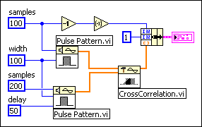
The following block diagram shows one way to index the CrossCorrelation VI.

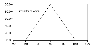
The following graph is the result of the preceding block diagram.

In order to make the cross correlation calculation more accurate, normalization is required in some situations. This VI provides biased and unbiased normalization.

1. Biased normalization
   
   If the normalization is biased, LabVIEW applies biased normalization as follows:
   
   

   R_xy(biased)_j =

   
   
   for j = 0, 1, 2, … , M+N–2
   
   where R_xy is the cross correlation between x and y with no normalization.
2. Unbiased normalization
   
   If the normalization is unbiased, LabVIEW applies unbiased normalization as follows:
   
   

   R_xy(unbiased)_j =

   
   
   for j = 0, 1, 2, … , M+N–2
   
   where R_xy is the cross correlation between x and y with no normalization. f(j) is:
   
   

   

2D Cross Correlation

The CrossCorrelation VI computes two-dimensional cross correlation as follows:

for i = –(M₁–1), … , –1, 0, 1, … , (M₂–1) and j = –(N₁–1), … , –1, 0, 1, … , (N₂–1)

where M₁ is the number of rows of matrix X,

N₁ is the number of columns of matrix X

,

M₂ is the number of rows of matrix Y

,

N₂ is the number of columns of matrix Y

,

the indexed elements outside the ranges of X and Y are equal to zero, as shown in the following relationships:

x(m,n) = 0, m < 0 or m M₁ or n < 0 or n N₁

and

y(m,n) = 0, m < 0 or m M₂ or n < 0 or n N₂.

The elements of the output matrix Rxy are related to the elements in h as follows:

R_xy(I,j) = h(i–(M₁–1), j–(N₁–1)) for i = 0, 1, 2, … , M₁+M₂–2 and j = 0, 1, 2, … , N₁+N₂–2.