Global Optimization VI

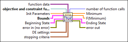
function data contains static data that the user-defined function needs at run time.

objective and constraint function is a reference to the VI that implements the nonlinear function, the nonlinear equality constraints function, and the nonlinear inequality constraints function as separate outputs. In the referenced VI, the objective function output must not be empty, but the constraint functions are optional. Therefore, the equality constraints output, the inequality constraints output, or both can be empty.

Create this VI by starting from the VI template located in labview\vi.lib\gmath\GlobalOptimization.llb\Global Optimization_Objective Function.vit.

Open template

Init Parameters are the initial parameters at which the optimization process starts. LabVIEW uses Init Parameters when Beginning State is empty. Each row of Init Parameters is one set of parameters. The number of columns in Init Parameters must equal the length of Min and Max in Bounds.

If the number of rows in Init Parameters is less than population size, LabVIEW initializes the remaining sets of parameters. If the number of rows in Init Parameters is larger than population size, LabVIEW ignores the additional sets of parameters.

Bounds is a cluster that contains the upper and lower numeric limits for the parameters being optimized.

	Min contains the lowest allowed value of the parameters being optimized. Min cannot be empty. The length of Min must be equal to the length of Max. Min does not accept exceptional values, such as Inf, –Inf, or NaN.
	Max contains the highest allowed value of the parameters being optimized. Max cannot be empty. The length of Max must be equal to the length of Min. Max does not accept exceptional values, such as Inf, –Inf, or NaN.

Beginning State contains the initial values of the populations and Pareto indexes. Beginning State is typically the ending state of a previous optimization and allows a warm start of the optimization. If Beginning State has values, LabVIEW ignores Init Parameters.

Population contains a set of parameters, which includes values of parameters, objective functions, equality constraints, inequality constraints, and the base index.

	Parameters contains the values of candidate parameters.
	Objective Functions contains the values of objective functions at Parameters.
	Equality Constraints contains the values of equality constraints at Parameters.
	Inequality Constraints contains the values of inequality constraints at Parameters.

Pareto Indexes contains index that determines the selection of parameters from all candidates.

error in describes error conditions that occur before this node runs. This input provides standard error in functionality.

DE Settings contains additional settings that are specific to the differential evolution (DE) method.

population size is the number of sets of candidate parameters that LabVIEW calculates at each loop iteration in the optimization process. This size also indicates the number of objective function calls at each loop iteration in the optimization process. A larger population size usually results in better optimization results and a longer execution time. The default is 10.

scale factor is the diversity factor that LabVIEW uses to generate mutant parameters. Larger values of scale factor result in more diverse mutant parameters. The default is 0.9.

crossover probability is the probability that LabVIEW inherits the trial parameters from the mutant parameters. A larger value of crossover probability results in a higher probability that LabVIEW accepts the mutant parameters. The default is 0.95.

bound mapping method is the method that LabVIEW maps the trial parameters into bounds.

0	None
1	Random between Bounds and Values (default)
2	Re-Initialize

mutation method is the method that LabVIEW generates mutant parameters.

0	Random (default)
1	Either Or
2	Best
3	Target to Best

crossover method is the method that LabVIEW crosses candidate parameters with mutant parameters.

0	Uniform (default)
1	Exponential

stopping criteria is the collection of conditions that terminate the optimization process.

	max iterations is the maximum number of loop iteration in the optimization process. If the number of loop iteration exceeds max iterations, the optimization process terminates. The default is 50.
	max function calls is the maximum number of objective function calls allowed before the optimization process terminates. The default is -1. -1 indicates that the optimization process never terminates and does not rely on the number of objective function calls. The formula that determines the actual number of objective function calls is population size * (max iterations + 1).
	max time (sec) is the maximum amount of time LabVIEW allows between the start and the end of the optimization process. The default is -1. -1 indicates that the optimization process never times out.

number of function calls is the number of times the objective function calls in the optimization process.

If max function calls is -1, number of function calls equals population size * (max iterations + 1).

Minimum is the determined global minimum among all minimum possibilities.

F(Minimum) is the function value of the objective function at Minimum.

Ending State contains the final values of the populations and Pareto indexes at the end of the optimization process.

Population contains a set of populations, which includes values of candidate parameters, objective functions, equality constraints, and inequality constraints at the end of the optimization process.

	Parameters contains the values of candidate parameters at the end of optimization process.
	Objective Functions contains the values of objective functions at Parameters.
	Equality Constraints contains the values of equality constraints at Parameters.
	Inequality Constraints contains the values of inequality constraints at Parameters.

Pareto Indexes contains the index that determines the selection of parameters from all candidates.

error out contains error information. This output provides standard error out functionality.

Global Optimization Details

This VI solves a global optimization equation by finding x to minimize f(x), which is subject to the following constraints:

Boundary constraints	min ≤ x ≤ max
Equality constraints	g(x) = 0
Inequality constraints	h(x) ≤ 0

x is the set of parameters to optimize. f(x) is the set of objective functions to minimize. The equality and inequality constraints are optional in this problem.

Differential evolution (DE) is one method used to solve the global optimization problem. It approximates the actual global optimum by iteratively mutating and improving the candidate parameters from the initial ones.

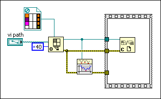
Note The DE method cannot guarantee the global optimum is found. The best parameters return depending on the choice of the DE settings as well as the problem itself.

If object function evaluation takes long time, the DE method needs to call the object function several times, depending on population size, during each loop iteration in the optimization process. This VI enables parallel loop iterations on the For Loop to call the object function so that LabVIEW can take advantage of multiple processors. In order to utilize the parallel loop iterations, you need to do the following:

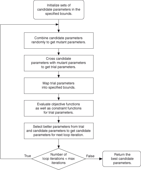
Change the VI that implements the objective function to a reentrant VI that shares clones.
Open a reference to a VI with a 0x40 option, as the following shown in the following image.

The following illustration shows how the VI solves a global optimization equation.

Examples

Refer to the following VIs for examples of using the Global Optimization VI:

Find Global Min on Surface VI: labview\examples\Mathematics\Optimization
Open example Find related examples
Two Circles Optimization VI: labview\examples\Mathematics\Optimization
Open example Find related examples