Spline Interpolation 1D VI

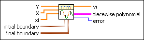
Y is the array of tabulated values of the dependent variable.

X is the array of tabulated values of the independent variable. The length of X must equal the length of Y.

xi is the array of values of the independent variable at which interpolated values of the dependent variable yi are to be computed.

initial boundary sets the conditions at the initial boundary.

boundary sets the boundary condition type. The default is natural spline.

0	natural spline—Specifies that the second derivative at the initial boundary is 0 and that LabVIEW ignores the derivative value input.
1	not-a-knot—Specifies that the third derivative at the second data point x₁ in X is continuous, which means this VI fits one polynomial through the first three data points, and the polynomial between [x₀, x₁] is the same as the polynomial between [x₁, x₂]. This option is useful if you know nothing about the derivatives at the initial boundary. If you specify not-a-knot, LabVIEW ignores the derivative value input.
2	1st derivative—Specifies that derivative value specifies the first derivative at the initial boundary.
3	2nd derivative—Specifies that derivative value specifies the second derivative at the initial boundary.

derivative value is the value of the first or second derivative at the initial boundary. This VI ignores derivative value when boundary is natural spline or not-a-knot.

final boundary sets the conditions at the final boundary.

boundary sets the boundary condition type. The default is natural spline.

0	natural spline—Specifies that the second derivative at the final boundary is 0 and that LabVIEW ignores the derivative value input.
1	not-a-knot—Specifies that the third derivate at the second-to-last data point in X, x_{n – 2}, is continuous, which means this VI fits one polynomial through the last three data points, and the polynomial between [x_{n – 2}, x_{n – 1}] is the same as the polynomial between [x_{n – 3}, x_{n – 2}]. This option is useful if you know nothing about the derivatives at the final boundary. If you specify not-a-knot, LabVIEW ignores the derivative value input.
2	1st derivative—Specifies that derivative value specifies the first derivative at the final boundary.
3	2nd derivative—Specifies that derivative value specifies the second derivative at the final boundary.

derivative value is the value of the first or second derivative at the final boundary. This VI ignores derivative value when boundary is natural spline or not-a-knot.

yi is the output array of interpolated values that correspond to the xi independent variable values.

piecewise polynomial is a cluster that contains the x locations and coefficients of the piecewise interpolating polynomial.

	x locations are the x domain endpoint values of the piecewise interpolating polynomial. If x locations is of size N, the coefficients array should contain N–1 rows of polynomial coefficients.
	coefficients is a 2D array of interpolating polynomial coefficients. Row i of coefficients contains the coefficients for the interpolating polynomial between elements x_i and x_i+1 of x locations.

error returns any error or warning from the VI. You can wire error to the Error Cluster From Error Code VI to convert the error code or warning into an error cluster.

Spline Interpolation 1D Details

The VI accepts tabulated X and Y values (independent and dependent variables, respectively) and provides interpolated values yi that correspond to each xi location. The VI looks up each value of xi in X and uses the relative location in X to find the interpolated value yi at the same relative location within Y.

The spline interpolation method guarantees that the first and second derivative of the piecewise interpolating polynomial are continuous, even at the data points.

In addition to the interpolated yi values, this VI also exports the piecewise polynomial cluster, which contains the piecewise x locations and corresponding polynomial coefficients used in the interpolation.

You can use the Evaluate Interpolating Polynomial VI to calculate the interpolated values using the piecewise polynomial.

Refer to A Practical Guide to Splines in the Mathematics Related Documentation topic for more information about the spline interpolation method.