Power Fit VI

Y is the array of dependent values. The length of Y must be greater than or equal to the number of unknown parameters.

X is the array of independent values. X must be the same size as Y.

Weight is the array of weights for the observations (X, Y). Weight must be the same size as Y. Weight also must contain non-zero elements. If an element in Weight is less than 0, the VI uses the absolute value of the element.

If you do not wire an input to Weight, the VI sets all elements of Weight to 1.

tolerance determines when to stop the iterative adjustment of amplitude, power, and offset. For the Least Square and Least Absolute Residual methods, if the relative difference between residue in two successive iterations is less than tolerance, this VI returns the resulting residue. For the Bisquare method, if any relative difference between amplitude, power, and offset in two successive iterations is less than tolerance, this VI returns the resulting amplitude, power, and offset.

If tolerance is less than or equal to 0, this VI sets tolerance to 0.0001.

method specifies the fitting method.

0	Least Square (default)
1	Least Absolute Residual
2	Bisquare

parameter bounds contains the upper and lower constraints for the amplitude, power, and offset. If you know the exact value of certain parameters, you can set the lower and upper bounds of those parameters equal to the known values.

	amp min specifies the lower bound for the amplitude. The default value is –Inf, which means no lower bound is imposed on the amplitude.
	amp max specifies the upper bound for the amplitude. The default value is Inf, which means no upper bound is imposed on the amplitude.
	power min specifies the lower bound for the power. The default value is –Inf, which means no lower bound is imposed on the power.
	power max specifies the upper bound for the power. The default value is Inf, which means no upper bound is imposed on the power.
	offset min specifies the lower bound for the offset. The default value is 0, which means the offset must be greater than or equal to 0.
	offset max specifies the upper bound for the offset. The default value is 0, which means the offset must be less than or equal to 0.

Best Power Fit returns the y-values of the fitted model.

amplitude returns the amplitude of the fitted model.

power returns the power of the fitted model.

offset returns the offset of the fitted model.

error returns any error or warning from the VI. You can wire error to the Error Cluster From Error Code VI to convert the error code or warning into an error cluster.

residue returns the weighted mean error of the fitted model. If method is Least Absolute Residual, residue is the weighted mean absolute error. Otherwise, residue is the weighted mean square error.

Power Fit Details

This VI uses the iterative general Least Square method and the Levenberg-Marquardt method to fit data to the power function of the general form described by the following equation:

f = ax^b + c

where x is the input sequence X, a is amplitude, b is power and c is offset. This VI finds the values of a, b, and c that best fit the observations (X, Y).

The following equation specifically describes the power function resulting from the general power fit algorithm:

y[i] = a(x[i])^b + c

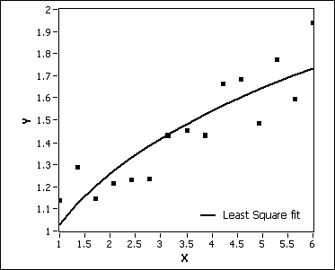
If the noise of Y is Gaussian distributed, use the Least Square method. The following illustration shows the power fit result using this method.

When you use the Least Square method, this VI finds the amplitude, power, and offset of the power model by minimizing residue according to the following equation:

where N is the length of Y, w_i is the i^th element of Weight, f_i is the i^th element of Best Power Fit, and y_i is the i^th element of Y.

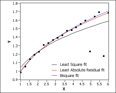
The Least Absolute Residual and Bisquare methods are robust fitting methods. Use these methods if outliers in the observations exist. The following illustration compares the fit results of the Least Square, Least Absolute Residual, and Bisquare fitting methods. In most cases, the Bisquare method is less sensitive to outliers than the Least Absolute Residual method.

When you use the Least Absolute Residual method, this VI finds the amplitude, power, and offset of the power model by minimizing residue according to the following equation:

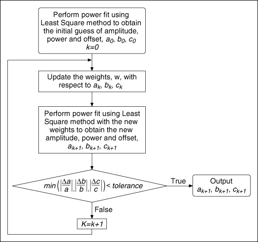
When you use the Bisquare method, this VI obtains the amplitude, power, and offset using an iterative process, as shown in the following illustration, and calculates residue using the same formula as the Least Square method.

Example

Refer to the Linear, Exp, and Power Fit VI in the labview\examples\Mathematics\Fitting directory for an example of using the Power Fit VI.

Open example Find related examples